3D Reconstruction: problems and solutions
Introduction
In this article we aim to introduce a possible solution for solving the 3D reconstruction problem. We will take advantage of the 3D Vision to reconstruct the object starting from a set Point Cloud which represents different views of the object. Firstly, we will start by detailing the difference between standard computer vision (2D) and 3D vision.
Secondly, we will detail the different stages of reconstruction, explaining a little bit about the algorithm used and different possible implementation choices. As a reference library, we are going to use the Point Cloud Library (PCL).
Lastly, we are going to create a full pipeline of registration.
2D Vision vs. 3D Vision
Most of the current applications work with standard 2D cameras. These cameras work by mapping the world they perceive in a discrete matrix, where each entry is called “pixel” and its color is obtained by adding three components Red, Green, Blue (from here RGB).
By definition, 2D cameras discard the depth of the images that they create. This does not mean that they cannot perceive 3D information, however, to achieve so, it is needed to perform a complex procedure called calibration.
The process of calibration consists in finding two sets of parameters:
- Intrinsics: A set of parameters that rectifies the distortion introduced by the lens
- Extrinsics: A set of parameters which represents the roto-translation to estimate the depth information in a 2D image given a calibration object as a reference
On the contrary, 3D cameras (in this article I will take as an assumption that we are talking about depth cameras that use LiDAR technology), perceive also depth information. The calculation to compute the depth information relies on Time of Flight (ToF) sensors.
The representation of the depth information can be represented in two different ways:
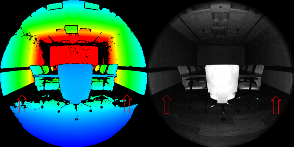
- Depth Map: Creation of a color map that represents the distances from the ToF sensor on the camera
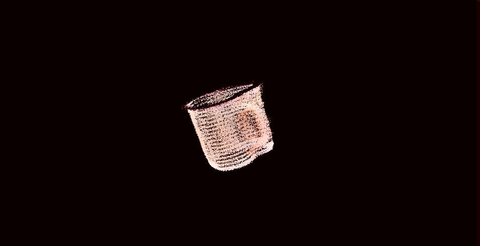
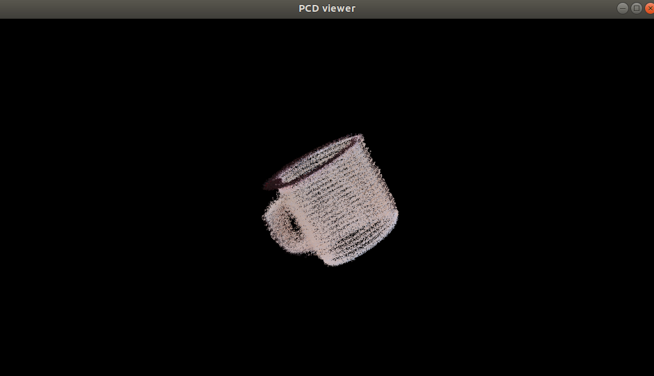
- Point Cloud: Creation of a set of points which represents our objects in a 3D scene (the representation used in this article)
Below are two images that represent the two concepts expressed in the previous lines:
The question which might arise is, why should I use a depth camera instead of a calibrated 2D camera? Are there any advantages?
In a nutshell, theoretically speaking there should be no differences between a depth camera and a 2D calibrated camera, however, it is generally preferred to obtain depth information from a sensor which in most applications is more precise than a calibration process.
From an algorithmic point of view, the operation working with 3D and 2D vision is significantly different.
2D images consist of a matrix of elements which are a composition of three components (RGB).
On the other hand, Point Clouds are a set of unordered points with spatial properties (and optionally others, like colors, normal, etc…), and thus require a completely different structure to work with.
Let’s be clear however on the tradeoff before moving on, depth cameras are more precise but they require higher computational complexity algorithms to work with.
Working with 3D Vision
Introduction
Most of the common 2D Vision applications work with a composition of linear(ized) systems or by correlating a matrix on the input image.
This approach works for both image elaboration (edge sharpening, noise removal etc…) and computer vision (feature extraction, pattern matching etc…).
In contrast with 2D Vision, 3D vision needs complex algorithms to work, spanning from complex non-linear systems to optimization algorithms.
In order to understand better we now detail some basic algorithms to have the reader get the picture on how to properly use this tool.
Filtering
We detail two types of algorithms, one for filtering outliers and one for downsampling:
- Statistical Outlier Removal: This algorithm selects a group of nearest points, with respect to a point and finds the mean and deviation of the distance of the points. If some points are above this threshold, they are discarded.
- VoxelGrid (for downsampling): This algorithm selects a group of nearest points, with respect to a point and finds the centroid. The points are replaced by the centroid.
These two algorithms introduce a common point, which is that in many cases the Point Cloud works with neighbours of points.
Normal estimation
Due to the fact that we are working with points that have spatial properties, it is possible to compute the normals of a point cloud. This is possible by grouping a set of points and estimating the normal. This computation also creates curvature information which is added to the Point Cloud. On the other hand of the other points shown above, this operation is considered an actual feature extractor, as it extracts new information out of the point cloud.
Normal estimation is probably the most useful task of the PCL, as it helps in performing the most important tasks such as segmentation, alignment, or triangulation.
KDTree
The Point Cloud representation brings with it an enormous problem, the points do not have any ordering property. This implies that there exists no efficient visit method (i.e. nearest point in space, which is the ordering we humans unconsciously apply to 3D objects). If there exists no visit method, any operation performed will be extremely expensive from a computational point of view.
To overcome this difficulty, PCL implements KDTree, which is a structure for ordering points in a K-dimensional space.
This structure is computed before most of the operations of the PCL in order to speed up computational time.
Segmentation
The segmentation operation in Point Cloud is equivalent to the one in 2D Vision. It consists of dividing the Point Cloud (or the image) into different regions. In the case of Point Cloud, it is usually used to separate the objects in the scene. There are three main types of segmentation techniques used in PCL:
- Clustering: This operation groups points that are near in space, and the generic technique used is clustering based on Euclidean distance.
- Region Growing: This segmentation method consists of grouping points that have a common property below a set threshold. For example one of the most commonly used is the Color Region Growing, which groups together points that have similar RGB intensity.
- Difference of Normals: This method relies on an assumption that is that the normal estimates of a group of points reflects the geometry underneath of the object. Thus a normalized difference should isolate different ROIs.
A completely different type of segmentation, used to segment specific shapes, is called Sample Consensus. PCL integrates an algorithm called RANSAC which is capable of segmenting different objects in a scene by fitting a parametric model of the object (3D Sphere, a Plane, a 3D Cylinder, etc…).
Alignment
The process of alignment consists in finding a roto-translation between two or more Point Clouds that minimizes the distance between shared points.
This process is similar to the one portrayed in 2D computer vision, therefore, it needs massive feature extraction to identify the common points based on features. The features are then used to compute the correspondence rejection (as in 2D computer vision), its covariance matrix and then the overall result is fitted with different possible methods.
The most commonly used algorithms are:
- ICP: A brute force approach to align Point Clouds by fitting the source into the target. It works properly if and only if the final transformation is a small roto-translation or if we have an initial guess.
- GICP: A more sophisticated version of the ICP which tries to find the correspondence to reject and then fit the source into the target.
- Normal Distribution Transform: Uses a function called score which tries to describe locally the normals in order to find with a non-linear optimizer the best transform to fit our alignment.
The process of the alignment in Point Cloud is definitely one of the most complex as it involves an enormous amount of non-linear operations.
Creation of a 3D registration pipeline
The last part of this article consists in using the previously shown operation to construct a robust registration pipeline.
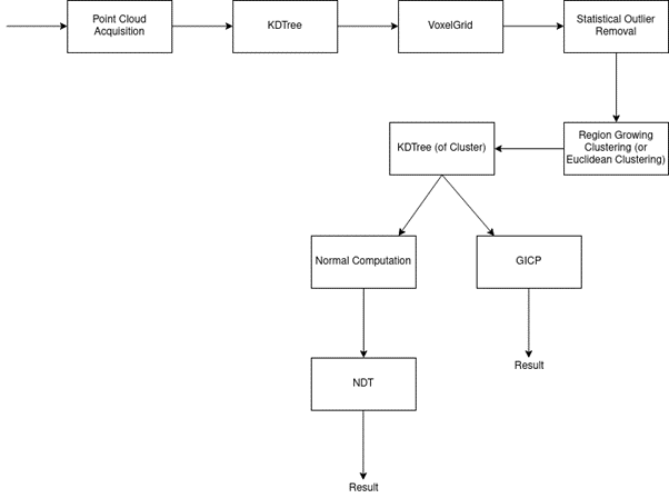
The idea of the pipeline should be the following:
- Acquisition of the Point Cloud
- Filtering and Downsampling (if Point Cloud is too dense)
- Clustering
- Cluster Extraction
- Alignment with a previous Point Cloud
- Transform the acquired Point Cloud into the target
- Come back to point 1.
The pipeline is then:
Conclusion
To conclude our brief journey into 3D Vision, let us remark on an important point. The set of algorithms introduced before requires an enormous amount of operations and thus to work with low latency applications they need some sort of acceleration or strong downsampling. The next article is going to cover a possible acceleration of the set of operations needed from the PCL to fit or solve complex systems.
Enjoy your acceleration