Path Following in AGV using Xilinx FPGAs
Introduction
This article introduce a possible architectural design for path planning for Autonomous Guided Vehicles (AGV).
The article proposes a set of functional blocks and their interaction to ensure Real-Time path planning on a Xilinx KRIA System On Module and Xilinx ZCU104.
The article is divided in four main sections:
- Modelling of the car-like system
- Setup of the system
- Trajectory Planning
- Proposed Architectural Design
Modelling of the car-like system
The modelization of the car-like is an interesting topic in Analytical Mechanics and Robotics, due the system being underactuated.
A mechanical system is said to be underactuated if its configurations are more than the ones that we can actually actuate. In this case the generated description of the model constraint, with respect to the configurations, involves also the generalized velocities.
In Analytical Mechanics the system is also usually referred to as non-holonomic.
We now give the system we use to describe the car-like system[1]:
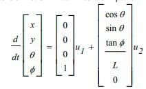
As it is easy to catch, the system is composed of four configurations, but we suppose our car is moving in a 2 dimensional space. Moreover, due to the property of being non-holonomic, we do not have a dynamical system describing it, but just a kinematical one, making the description harder than usual. We now give a simple draft of the car, in order to clarify the meaning of the whole components of the formula given[1]:
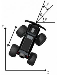
The four variables in the system then are:
- X: The X coordinate of our imaginary plan where the car is moving
- Y: The Y coordinate of our imaginary plan where the car is moving
- Θ: The actual steering angle taking in account the L factor (the distance between steering and rear wheels)
- ɸ: The desired angle which we would like the car to steer
The above description of the car-like system can be used to represent and integrate our system with respect to a specific trajectory which we want the AGV to follow.
At the end of the chapter it is underlined that the proposed model is simpler than the ones actually used in commercial application, and used with the only aim of making the reader comprehending the basics of non-holonomic modelling. For this reason the reader is encouraged in further readings.
Setup of the system
Our autonomous vehicle needs to be compliant with the standard structure of agents that we use in ML & AI:
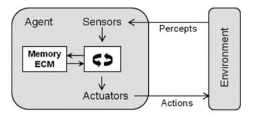
The scheme to follow is always fixed:
- The robot uses sensor to percept the surrounding environment
- It transforms the environment representation using some algorithms into actions
- Send command to the actuator based on the result the actions chosen
Following the three points above, in this chapter it is introduced the actuators and sensors used.
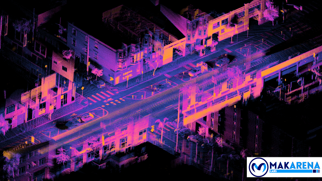
As sensors we will use LiDAR cameras, which will be placed on the AGV. The LiDAR cameras are a particular type of sensor which are able to create a depth mapping of the environment. A depth map consists in associating to every pixel of the image a distance, measured by the LiDAR sensor present in the camera. Following a visual example:
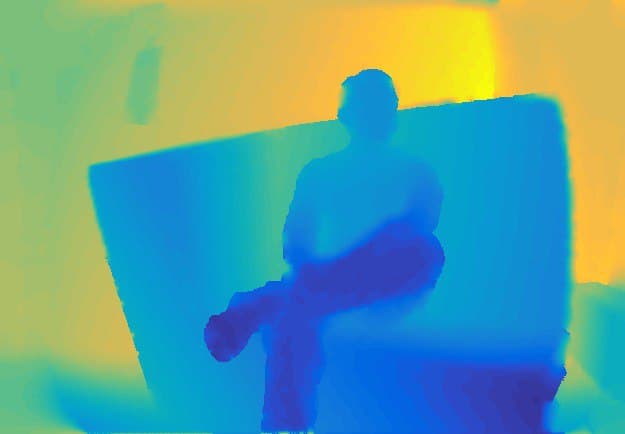
The image is a painted depth map [3], the cold colors represent the points closest to the camera, while the shading to the hot colors represents the points that are the ones farthest from the camera itself.
This description of the environment can be transformed into the well known Point Cloud. The Point Cloud is a description of the environment where we associate to every object a set of points to describe its shape and distance with respect to the camera, following an example:
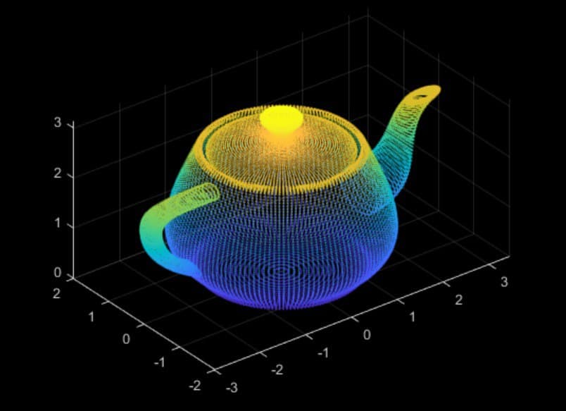
In our example application we will tend to use the Point Cloud description, due the versatility and power of the Point Cloud Library, an open-source tool created to perform operations on Point Cloud (i.e.: segmentation, clustering, alignment etc…).
Supposing our car can fit into a rectangle, we will place a camera for every side, which will allow us to locate the position of the car with respect to every direction in the environment.
The last point to discuss in our setup are the actuators. Ideally we will have 3 PMSM motors, one for the steering wheels and two for the rear wheels (we suppose rear-wheel drive for our system). Our motors will be controlled using Field Oriented Control (FOC). We will make use of the Xilinx Open-source project for controlling Electrical Drives called SPYN [4].
Our car is now set up, we proceed in the next chapter detailing the Trajectory Planning, but most important the obstacle avoidance technique used.
Trajectory Planning
Before detailing the trajectory planning part, we have skipped an important step in the car modelling, or rather its controllability. The controllability of the car is obtained with an instrument of the differential geometry called Lie Derivative [1].
Assuming that the system is controllable, and with no slip (the constraint of the system), we now dig a little bit in the trajectory planning for the car.
Before we have introduced the fact that we would have used the point cloud to represent our environment. This choice has been done for two specific reason:
- With Point Cloud we can implement SLAM (Simultaneous Localization And Mapping) techniques, which consists in the updating of the known environment of the vehicle using a probabilistic approach based on the system inputs and previous locations.
- We can make use of Machine Learning to create models which segment what is present in a specific Point Cloud.
These two assumptions will be sufficient to create an AGV which must execute carriage tasks (i.e. in a factory or a logistic site). Our vehicle then must move from a point A to a point B, autonomously and possibly understanding critical situations.
If our environment is free from any obstacle, we can simply use the modelling system and SLAM to create a safe path from point A to point B, without any additional effort apart from setting up a proper controller. But in actual applications the environment evolves in a not predictable way, and thus we need an algorithm to perform obstacle avoidance.
In this article we do not treat Reinforcement Learning or Imitation Learning (which could be two good choices for this problem), if the reader would like to understand more about them, it is suggested to read a previous article on Learning methods for robots [5].
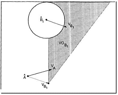
The algorithm chosen for obstacle avoidance is called Velocity Obstacle [6]. Let me suppose our car moves with a certain velocity in a certain direction. At a certain point in time, our system detects an obstacle (we will come back later on how we can detect it). If the obstacle is moving within our reference trajectory we must avoid it, otherwise a collision will take place, to have a better understand, it is left an image from the article where the technique is explained [6]:
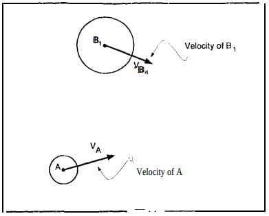
Our car is body A, whereas the obstacle is body B. The two estimated velocities will definitely bring a collision. How can we avoid body B?
The proposed method consists in 3 steps:
- Projecting the space configuration of our body A into the obstacle, enlarging it by the space configuration of body A
- The creation of a cone of forbidden velocities, which will represent our velocity obstacle
- The computation of the avoidance maneuver
Point 1 can be obtained thanks to our Point Cloud representation of the system, which can be used to estimate the space configuration of the obstacle, which from a geometrical point of view after the transformation is [6]:
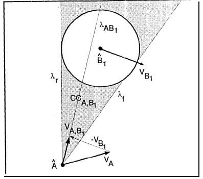
The picture above represents the projection of our body A into body B. Moreover it represents how we compute the cone of forbidden velocities, thanks to velocity vectors A and B (by an algebraic subtraction between the two), which will result in a cone. This cone is actually our velocity obstacle [6]:
The computation of the avoidance maneuver shown in the article is a heuristic search of a tree of possible maneuvers. The reader may use whatever techniques likes, as in the last years a lot of improvements on obstacle avoidance have been done in the robotic community and literature.
The last point to enlighten before moving on the architectural design on FPGA is how we can segment the obstacles.
The obstacle segmentation is done using a CNN on the Point Cloud of the environment. The CNN takes in input the Point Cloud of the environment and returns the elements which that compose the specific scene, following an example from Stanford University [7]:
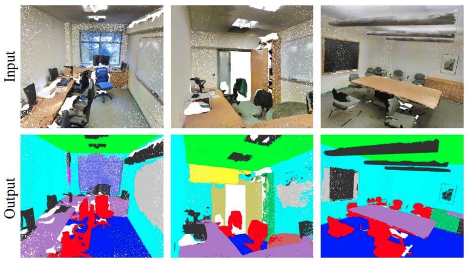
The power of Point Cloud is that with a segmentation of the scene it is possible to understand also the actual coordinates of the objects and not only what is, thanks to the representation of the actual space composition of the scene.
Xilinx supports CNN computation with the DPU (Deep Learning Processing Unit), a powerful already made IP that infer AI models from the most famous frameworks, such as Caffe, Tensorflow, Keras, PyTorch etc…
Proposed Architectural Design
Before giving the diagram of composition of the design, let us recall the components we need:
- A motor control IP, for actuation
- A set of drivers or IP block, to take input from camera
- A SLAM IP, for parsing Point Cloud and saving the environment discover
- A DPU IP, used to infer the CNN which segments the Point Cloud
- An IP for computing the velocity obstacles of the environment
- An IP for computing the chosen avoidance maneuver
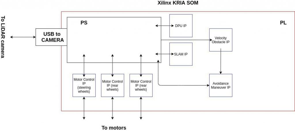
The high level results in:
- The PS (Processor A53) takes the depth image as input from the USB, and pass it to the SLAM IP to refresh the environment and the DPU to segment the object in the scene
- If no obstacle are encountered, then give commands to the actuators to follow the path
- If there is an update of the environment which includes obstacles to avoid (i.e. humans), the PS passes the coordinates of the objects to the Velocity obstacle IP and has as a result the velocity to apply to the actuators to avoid it.
- Continue from point 1.
AGV applications relies a lot on massive computations (i.e. CNN or Point Cloud with hundreds of thousands of points), for this reason the flexible acceleration architecture provided by FPGA will suit all the different IPs needed. Moreover the PL part of FPGA guarantees deterministic latency, and so the execution of the whole process can be guaranteed up to some check errors from the Cortex A53 in the Processing System.
Conclusions
In this article we have introduced a possible approach to path following for an AGV. The reader may find interesting the other references left, to have a clearer idea of the whole picture and not only what used in this article.
Enjoy your acceleration
Resources
[3] https://it.mathworks.com/matlabcentral/fileexchange/64546-depth-map-inpainting
[4] https://github.com/Xilinx/IIoT-SPYN
[5] https://www.makarenalabs.com/a-discussion-of-learning-algorithms-for-robotic-application/
[6] https://trs.jpl.nasa.gov/bitstream/handle/2014/32056/95-1447.pdf?sequence=1
[7] https://web.stanford.edu/~rqi/pointnet/docs/cvpr17_pointnet_slides.pdf